Differential Equation Identifier

What This Tool Does

The Differential Equation Identifier is a powerful Calculus utility that analyzes your equation and determines the correct solving method. It checks for linearity, separability, exactness, homogeneity, Bernoulli structure, and second-order patterns.

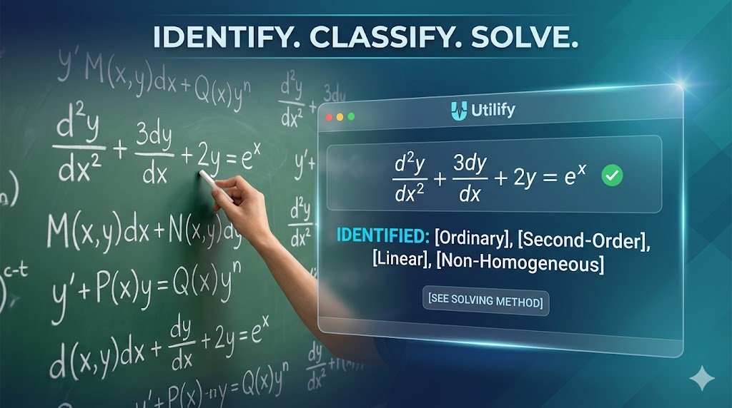
Paste your differential equation into the differential equation identifier below, or choose its form to see exactly what type it is and which method applies.

Common Differential Equation Identifier Types

Exact

These equations come from a hidden potential function, and checking exactness tells you whether the equation can be solved by direct integration. As always, the Differential Equations Identifier will help with all of these methods.

Form: M(x, y) + N(x, y) y’ = 0
How to recognize: The partial derivative of M with respect to y equals the partial derivative of N with respect to x.
Method: Integrate M with respect to x or N with respect to y.
Why it works: Exact equations come from a potential function whose total derivative is zero.

Example:
(2 x y + 3) + (x squared + 4 y) y’ = 0
Step 1: M equals 2 x y plus 3. N equals x squared plus 4 y.
Step 2: Check exactness: M sub y equals 2 x. N sub x equals 2 x. They match.
Step 3: Integrate M with respect to x: psi equals x squared y plus 3 x plus h of y.
Step 4: Differentiate psi with respect to y: x squared plus h prime of y equals x squared plus 4 y.
Step 5: Solve for h: h prime equals 4 y, so h equals 2 y squared.
Step 6: Final implicit solution: x squared y plus 3 x plus 2 y squared equals C.

Homogeneous

These equations depend only on the ratio y over x, and a simple substitution turns them into a separable equation.

Form: y’ = F(y over x)
How to recognize: Replacing x with t x and y with t y leaves the equation unchanged.
Method: Use substitution v equals y over x.
Why it works: The substitution reduces the equation to a separable form.

Example:
y’ = (x + y) divided by (x minus y)
Step 1: Substitute v equals y over x, so y equals v x and y’ equals v plus x v’.
Step 2: Substitute into equation: v plus x v’ equals (1 plus v) divided by (1 minus v).
Step 3: Solve for v’: x v’ equals (1 plus v squared) divided by (1 minus v).
Step 4: Separate: (1 minus v) over (1 plus v squared) dv equals dx over x.
Step 5: Integrate both sides: arctangent of v minus one half natural log of (1 plus v squared) equals natural log of absolute x plus C.
Step 6: Substitute v equals y over x back in.

Bernoulli

These equations look almost linear but include y raised to a power, and a substitution converts them into a standard linear form.

Form: y’ + P(x)y = Q(x) y to the n
How to recognize: It looks like a linear equation but has y to the n.
Method: Use substitution v = y to the power (1 minus n).
Why it works: The substitution turns it into a linear equation.

Example:
y’ + y = y squared
Step 1: This is Bernoulli with n = 2.
Step 2: Substitute v equals y to the negative one, which is one over y.
Step 3: Compute v’: v’ equals negative y’ over y squared.
Step 4: Substitute into equation to get v’ minus v equals negative one.
Step 5: Solve linear equation: integrating factor equals e to the negative x.
Step 6: Solve: v equals 1 plus C e to the x.
Step 7: Substitute back: one over y equals 1 plus C e to the x.
Step 8: Final solution: y equals 1 divided by (1 plus C e to the x).

Second‑Order Linear (Homogeneous)

These equations involve y, y’, and y” in a linear combination, and their solutions come from the roots of the characteristic equation.

Form: a y double prime + b y’ + c y = 0
How to recognize: Second‑order, linear, equals zero.
Method: Solve the characteristic equation.
Why it works: Solutions are combinations of exponentials based on the roots.

Example:
y double prime + 3 y’ + 2 y = 0
Step 1: Characteristic equation: r squared + 3 r + 2 = 0.
Step 2: Factor: (r + 1)(r + 2) = 0.
Step 3: Roots are r = negative 1 and r = negative 2.
Step 4: Solution: y = C1 e to the negative x plus C2 e to the negative 2x.

Non‑Homogeneous (Second‑Order)

These equations combine the homogeneous solution with a particular solution that matches the forcing function on the right side.

Form: a y double prime + b y’ + c y = f(x)
How to recognize: Same as homogeneous but with a forcing function.
Method: Complementary solution plus particular solution.
Why it works: The general solution is the sum of the homogeneous solution and one specific particular solution.

Example:
y double prime + 3 y’ + 2 y = e to the x
Step 1: Solve homogeneous part: r squared + 3 r + 2 = 0 gives r = negative 1 and negative 2.
Step 2: Complementary solution: y sub c = C1 e to the negative x plus C2 e to the negative 2x.
Step 3: Try particular solution y sub p = A e to the x.
Step 4: Substitute: A + 3 A + 2 A = 1 gives 6 A = 1, so A = one sixth.
Step 5: General solution: y = C1 e to the negative x + C2 e to the negative 2x + one sixth e to the x.

Laplace Transform Problems

These equations often include step functions or impulses, and the Laplace transform turns them into algebraic equations that are easier to solve.

Form: Often involve step functions, discontinuous functions, or delta functions.
How to recognize: You see u(t minus a), delta spikes, or piecewise forcing.
Method: Take Laplace transform, solve algebraic equation, then inverse transform.
Why it works: Laplace converts differential equations into algebraic equations.

Example:
y double prime + y = u(t minus 3), with y(0) = 0 and y'(0) = 0
Step 1: Laplace transform: (s squared + 1) Y(s) = e to the negative 3s divided by s.
Step 2: Solve for Y(s): Y(s) = e to the negative 3s divided by (s times (s squared + 1)).
Step 3: Factor out shift: Y(s) = e to the negative 3s times [1 divided by (s times (s squared + 1))].
Step 4: Partial fractions: 1 divided by (s times (s squared + 1)) equals 1 over s minus s over (s squared + 1).
Step 5: Inverse Laplace: f(t) = 1 minus cosine of t.
Step 6: Apply shift: y(t) = u(t minus 3) times [1 minus cosine of (t minus 3)].

FAQ

How does this differential equation Identifier determine the equation type?
It analyzes the structure of the equation, checking for patterns such as linearity, separability, exactness, homogeneity, or the presence of higher‑order derivatives.
Does this tool solve the equation for me?
No. It identifies the correct method and provides examples so you can solve it yourself.
Can I enter any differential equation?
The Differential Equation Identifier tool recognizes the most common types taught in first‑ and second‑year calculus and differential equations courses.

Thank you

Thank you for using the differential equation identifier! Keep checking back for further updates.